:
Due: , 11:59 pm
Objectives
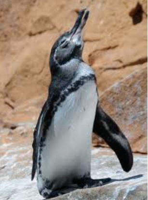 For project 4, we're going to move to the world of ecological modeling.
In particular, we're going to model the change in the population of
Galapagos Penguins over time, given certain ecological pressures. Our
goal is to model the risk of extinction over some number of years.
The model we will use is fairly simple, but you can choose to add
complexity to the model once the basic system is working.
For project 4, we're going to move to the world of ecological modeling.
In particular, we're going to model the change in the population of
Galapagos Penguins over time, given certain ecological pressures. Our
goal is to model the risk of extinction over some number of years.
The model we will use is fairly simple, but you can choose to add
complexity to the model once the basic system is working.
One new aspect for this project is the use of random values in the simulation. Because the world doesn't exhibit strong regularity, we're going to model this uncertainty by using a random number generator. For example, El Niño, an important weather factor in Galapagos Penguin survival, does not occur on a perfectly regular schedule, but it does tend to occur at least once every 5-7 years. We can model this by assigning a 1.0/5.0 or 1.0/7.0 probability of an El Niño to any given year. Then, each year of the simulation, we effectively roll a 5-sided or a 7-sided die and declare an El Niño year if it comes up with a 1. If the year is an El Niño year, then the penguin population drops significantly. If it is not an El Niño year, the population sees a small amount of growth.
Because of the random variables in the model, each time we model 100 years the computer will generate a different result. In one simulation, the population may go extinct in 20 years, in another simulation it may not go extinct at all. In order to achieve a reasonable estimate of the true probability of extinction over 100 years, we have to run the simulation many, many times and aggregate the results. For example, the probability of extinction in 100 years would be calculated as the number of simulations where the population goes extinct, divided by the total number of simulations. Researchers using simulation to evaluate the risk of extinction in actual populations might run the simulation a million times or more in order to get a stable estimate of extinction risk. Stability, in this case, means that if you run the simulation 1,000,000 times, then the difference between that average and the average of a different run of 1,000,000 simulations will be small.
To design the simulation, we're going to use hierarchical, modular design to keep each function simple to write and debug. Think about the project as having layers. The top layer is the controlling function and contains three parts. The first part sets up the parameters for the simulation. The second part runs the complete simulation many times and stores the results. The third part analyzes the results and generates the desired outputs.
The next layer down handles running a single simulation over numYears years. The full simulation function has two main parts. First, it sets up the initial population, then it simulates numYears years using a loop. It returns either the year in which the population went extinct or numYears if the population is still viable at the end of the simulation.
The bottom layer handles simulating a single year of the simulation. It takes in the current population and the ecological parameters and determines how many individuals are in the next year's population. It then returns the new population.
By designing the simulation in this manner, each function is well-defined and simple to write and debug. The tasks below provide more details on each level and the overall task.
Tasks
Setting Up
If you haven't already set yourself up for working on the project, then do so now:
- Mount your directory on the Personal server.
- Open the Terminal and navigate to your project4 directory on the Personal server.
- Open TextWrangler. If you want to look at any of the files you have already created, then open those files.
Create penguin.py
Create a new file penguin.py. For this week, all of the simulation functions will be in this file, though you can use the functions in your stats.py file to analyze the results, if you choose to pursue one of those extensions.
initPopulation( )
Create a function initPopulation(), which takes in two parameters: the initial population size (call it size), and the probability of an individual being female. The function should return a list of the specified size. Each entry in the list will be either an f or an m.
The function should first initialize a variable (e.g. population) to the empty list. Then it should use a loop to append size items to this list. Each time through the loop it should generate a random number using random.random(), which generates values between 0 and 1. If the value is less than the probability of an individual being female, append an f to the population list. Otherwise, append an m to the population list. Finally, return the population list.
You can use the following test function to see if your initPopulation() function is doing the right thing. It should print out a list of 10 individuals with an appropriate mix of f and m elements. Run it a few times to make sure you're getting randomized lists.
# test function for initPopulation
def test():
    popsize = 10
    probFemale = 0.5

    pop = initPopulation(popsize, probFemale)

    print pop

if __name__ == "__main__":
    test()
simulateYear( )
Create a function simulateYear() with six parameters:
- pop: the population list
- probFemale: the probability of a new individual being female,
- elNinoProb: the probability of an El Niño
- stdRho: the growth factor in a regular year. This number is meant to allow the population to grow each year and is expected to be greater than 1 (but less than or equal to 2).
- elNinoRho: the growth factor in an El Niño year. This number is meant to reduce the population and is therefore less than 1 (but greater than or equal to 0).
- maxCapacity: the max carrying capacity of the ecosystem.
The first step in the function is to determine if it is an El Niño year. Set a variable (e.g. elNinoYear) to False. Then compare the result of random.random() to the El Niño probability. If the random.random() result is less, then set elNinoYear to True.
The second part of the function is a loop over the existing population list. Before starting the loop, create a newpop list and set it to the empty list. Inside the loop, implement the following algorithm.
# for each penguin in the original population list
    # if the length of the new population list is greater than or equal to maxCapacity
        # break, since we don't want to make any more penguins

    # if it is an El Nino year
        # if random.random() is less than the El Nino growth/reduction factor
            # append the penguin to the new population list
    # else
        # append the penguin to the new population list
        # if random.random() is less than the standard growth factor - 1.0
            # if random.random() is less than the probability of a female
                # append an 'f' to the new population list
            # else
                # append an 'm' to the new population list
Finally, return the new population list.
To test your simulateYear() function, add the following code to your test function.
newpop = simulateYear(pop, 0.5, 1.0, 1.188, 0.4, 2000)

print("El Nino year")
print(newpop)

newpop = simulateYear(pop, 0.5, 0.0, 1.188, 0.4, 2000)

print("Standard year")
print(newpop)
You should see the population reduce to 3-6 individuals in the El Niño year and grow to 11-14 individuals in the standard year. Run it a few times to see the variation.
runSimulation( )
The next step is to write the runSimulation() function. This function takes in 8 parameters. You can use the definition below, if you wish, but feel free to modify the parameter names to ones that might be more clear to you.
def runSimulation( numYears, initPopSize, probFemale, elNinoProb, stdRho,
                    elNinoRho, maxCapacity, minViable ):
The function should first assign to a variable (e.g. population) the result of calling initPopulation with the appropriate arguments. Then it should set another variable (e.g. endDate) to numYears (the number of years to run the simulation). The variable endDate will be what the function returns.
The main part of the function should be a loop that runs numYears times. Each time through the loop it should call simulateYear() with the appropriate arguments, assigning the result to a new list variable (e.g. newPopulation). Then it should test if there are enough individuals in the new population list to be a viable population. It should also test if there are no males or no females in the new population list. If any of these tests fails, then set endDate to the loop variable value and break out of the loop. The final step in the loop is to assign to the population variable the newPopulation variable, replacing the old population with the new one.
If you want to graph or view the population numbers over time, print out the length of the population list at the end of each loop. Alternatively, you could save the numbers to a file.
Add some test code to your test function that calls runSimulation() a few times with some appropriate arguments. Make sure the initPopSize argument is larger than the minViable argument.
Default values for the simulation are as follows:
| numYears | 201 | |
|---|---|---|
| Initial Population Size | 500 | |
| Probability of Females | 0.5 | |
| Probability of an El Niño | 1.0/7.0 | |
| Growth Factor in a standard year | 1.188 | |
| Growth Factor in an El Niño year | 0.41 | |
| Maximum Carrying Capacity | 2000 | |
| Minimum Viable Population | 10 |
Use these values unless any of them are superseded by user input. (For example, in the next section, you'll be instructed to write code that will take command-line input containing the number of years between El Niño events. In that case, use the input value to come up with the probability of an El Niño, and disregard the default.)
main( )
The top level function is your main function. Give it one argument, argv, which will be the list of strings from the command line.
Start your main function by testing if there are three arguments on the command line. The first argument will be the name of the program, the second should be the number of simulations to run, and the third should be the typical number of years between an El Niño event. If there are less than three (len(argv) < 3), print out a usage statement and exit.
After the test for arguments, cast the second argument (argv[1]) to an integer and assign it to a variable that specifies the number of simulations to run (e.g. numSim). Cast the third argument (argv[2]) to an integer and assign it to a variable that specifies the typical number of years between an El Niño event.
In the next section of your program, create variables for each of the simulation parameters in the table above not already assigned and give them the default values. You should also create a variable to hold the results of the simulations and initialize it to the empty list.
Loop over the number of simulations. Inside the loop, append to your result list the result of calling runSimulation() with the appropriate arguments.
Finally, count how many of the results in your result list are less than numYears (the number of years to simulate). Divide that count by the total number of simulations and print out the result. This is the overall probability that the penguins will go extinct within the next numYears years.
Run your program using 100 simulations and see what you get. Does it change a lot? Run it with 1000 simulations (which might take a little while) and see if the results are more stable.
computeCEPD( )
The next task is to write a function that takes the list of results,
which is a set of numbers indicating the last year in which the
population was viable, and convert it to a
The computeCEPD() function should take two arguments: the list of results from runSimulation() (a list of integers), and the number of years the simulation ran (numYears).
The computeCEPD() function has three parts.
- The first part is to create a list (e.g. CEPD) with numYears zeros. You can do this by appending numYears zeros to an empty list in a loop.
- The second part is to loop over the list of results (extinction years). If the extinction year is less than numYears, loop from the extinction year to numYears and add one to each of those entries in the CEPD list.
- The third part is to loop over the CEPD list and divide each entry by the length of the extinction year results list, which is also the number of simulations. After this, return the CEPD list.
Add a call to the computeCEPD() function to the end of your top level function. Then have your top level function print out every 10th entry in the CEPD list (remember how the range function works). Run your penguin simulation 1000 times using the standard parameters. Repeat the process three times and show the results in your writeup. How much variation is there in the results?
Analysis
The final step is to use your simulation to compare the extinction distribution curves for a 3-year El Niño cycle, a 5-year El Niño cycle, and a 7-year cycle. What do your results indicate?
Extensions
Each assignment will have a set of suggested extensions. The required tasks and writeup constitute about 83% of the assignment. If you do only the required tasks and writeup -- and do them well -- you will earn a B. To earn a higher grade, you need to undertake one or more extensions. The difficulty and quality of the extension or extensions will determine your final grade for the assignment. One complex extension, done well, or 2-3 simple extensions are typical.
These are only examples to help you start thinking of the unlimited possible ways you could extend the project. You are strongly encouraged to design your own extensions to suit your interests and show off your computational thinking skills.
Whichever extensions you choose, be sure to discuss your motivation, design process, implementation, and results in the writeup. A screenshot of your results is usually a great idea.
Add other model parameters to the command line. The complex version of this extension is to have flags for your program so that the user can use a flag, like -E, to specify a given parameter. For example, running
python3 penguin.py -E 5would modify the El Niño frequency but leave all other parameters at their default values.
- Display the CEPD data in a graph. Adjust the code in penguin.py so that it prints out the year and CEPD for all years. Redirect the output to a .csv file. Use Excel or other software to plot the data and post the image on the wiki with a thorough description of its contents.
- Explore variations on the model. For example, what effect on the extinction probability do you see if you adjust the number of years in the El Niño cycle? Does changing the carrying capacity to 3000, for example, modify the 100-year extinction probability for the 5 year El Niño cycle?
- More rigorously test the variation in the simulation outcomes. Use your standard deviation function to compare the standard deviation of the probability that the population goes extinct at a particular time. For example, consider 200 years when the El Niño cycle is 5 years. Running the simulation with numSim=100 will likely yield a larger standard deviation in the values of the CEPD at t=200 (the final year of the simulation) than running the simulation with numSim=1000 will.
- Figure out the complexity of the simulation as a function of the parameters. How many times does the main loop in runSimulation() execute, on average?
Write Up & Hand In
Turn in your code by putting it into your private hand-in directory on the Courses server. All files should be organized in a folder titled Project 4 and you should include only those files necessary to run the program. We will grade all files turned in, so please do not turn in old, non-working, versions of files.
Make a new wiki page for your assignment. Put the label cs152f18project4 in the label field on the bottom of the page, and give the page a meaningful title (e.g. Eric's Project 4).
In general, your intended audience for your write-up is your peers not in the class. Your goal should be to be able to use it to explain to friends what you accomplished in this project and to give them a sense of how you did it. Follow the outline below.
- Title includes your name and clearly describes the project.
- Section headings are used to delineate distinct sections of the report.
- Abstract identifies key lecture concepts (e.g. code structures, data types, and libraries) relevant to the project.
- Abstract explains why key lecture concepts are important to achieving project goals.
- Abstract identifies program output(s), giving context to the project tasks.
- Solutions to tasks are described, focusing on how you used key lecture concepts to solve each task.
- Required images/outputs are present and clearly labeled.
- Reflection at the end of the report addresses how the lecture concepts mentioned in the abstract made this project possible. If you can think of a more elegant way to achieve the same results, please share!
- Sources, imported libraries, and collaborators are cited, or a note is included indicating that none were referenced.
- Double-check this week's label. Make sure it is there.
Thanks to Cathy Collins for the project idea and documentation. The original project concept and idea came from "Problem-Solving in Conservation Biology and Wildlife Management, 2nd Edition", by James P. Gibbs, Malcolm L. Hunter, Jr., Eleanor J. Sterling.
© 2019 Eric Aaron (with contributions from Colby CS colleagues).